A reliable transport protocol

A simple reliable protocol

In this section, we develop a simple reliable protocol running above the network service. To design this protocol, we first assume that the underlying layer provides a perfect service. We will then develop solutions to recover from different types of errors that affect the network service.

The network layer is designed to send and receive packets on behalf of a user. We model these interactions by using the DATA.req and DATA.ind primitives. However, to simplify the presentation and to avoid confusion between a DATA.req primitive issued by the user of the network layer, and a DATA.req issued by the transport layer entity itself, we use the following terminology :

• the interactions between the user and the transport layer entity are represented by using the classical DATA.req and the DATA.ind primitives

• the interactions between the transport layer entity and the sub-layer are represented by using send instead of DATA.req and recvd instead of DATA.ind

When running on top of a perfect network, a transport entity can simply issue a send(SDU) upon arrival of a DATA.req(SDU) [1]. Similarly, the receiver issues a DATA.ind(SDU) upon receipt of a recvd(SDU). Such a simple protocol is sufficient when a single SDU is sent. This is illustrated in the figure below.

Unfortunately, this is not always sufficient to ensure a reliable delivery of SDUs. Consider the case where a client sends tens of SDUs to a server. If the server is faster than the client, it will be able to receive and process all the segments sent by the client and deliver their content to its user. However, if the server is slower than the client, problems may arise. The transport entity contains buffers to store SDUs that have been received as a Data.request but have not yet been sent. If the application is faster than the network, the buffer may become full. At this point, the operating system suspends the application to let the transport entity empty its transmission queue. The transport entity also uses a buffer to store the received segments that have not yet been processed by the application. If the application is slow to process the data, this buffer may overflow and the transport entity will not able to accept any additional segment. The buffers of the transport entity have a limited size and if they overflow, the arriving segments will be discarded, even if they are correct.

To solve this problem, a reliable protocol must include a feedback mechanism that allows the receiver to inform the sender that it has processed a segment and that another one can be sent. This feedback is required even though there are no transmission errors. To include such a feedback, our reliable protocol must process two types of segments :

• data segments carrying a SDU

• control segments confirming that the previous segment was correctly processed

These control segments are usually called acknowledgments because they acknowledge the correct reception of data.

These two types of segments can be distinguished by dividing the segments in two parts :

• the header that contains a segment type bit set to 0 in data segments and set to 1 in control segments

• the payload that contains the SDU supplied by the application

Our transport entity can then be modeled as a finite state machine, containing two states for the receiver and two states for the sender. Fig. 47 provides a graphical representation of this state machine with the sender above and the receiver below.

Fig. 47 Finite state machines of the simplest reliable protocol (sender above, receiver below)

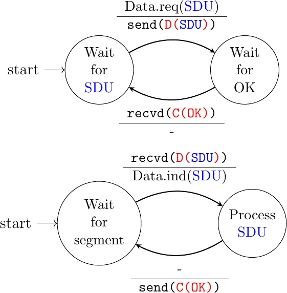
The sender FSM shows that the sender has to wait for an acknowledgment from the receiver before being able to transmit the next SDU. The figure below illustrates the exchange of a few segments between two hosts.

Note

Services and protocols

An important aspect to understand when studying computer networks is the difference between a service and a protocol. For this, it is useful to start with real world examples. The traditional Post provides a service where a postman delivers letters to recipients. The Post precisely defines which types of letters (size, weight, etc) can be delivered by using the Standard Mail service. Furthermore, the format of the envelope is specified (position of the sender and recipient addresses, position of the stamp). Someone who wants to send a letter must either place the letter at a Post Office or inside one of the dedicated mailboxes. The letter will then be collected and delivered to its final recipient. Note that for the regular service the Post usually does not guarantee the delivery of each particular letter. Some letters may be lost, and some letters are delivered to the wrong mailbox. If a letter is important, then the sender can use the registered service to ensure that the letter will be delivered to its recipient. Some Post services also provide an acknowledged service or an express mail service that is faster than the regular service.

Reliable transfer above an imperfect link

The transport layer must deal with several types of errors which can affect the segments that it sends. In practice, we mainly have to deal with two types of errors in the transport layer :

• Segments can be corrupted by transmission errors

• Segments can be lost or unexpected segments can appear

To detect errors, a segment is usually divided into two parts :

• a header that contains the fields used by the reliable protocol to ensure reliable delivery. The header contains a checksum or Cyclical Redundancy Check (CRC) [Williams1993] that is used to detect transmission errors

• a payload that contains the user data

Some headers also include a length field, which indicates the total length of the segment or the length of the payload.

The simplest error detection scheme is the checksum. A checksum is basically an arithmetic sum of all the bytes that a segment is composed of. There are different types of checksums. For example, an eight bit checksum can be computed as the arithmetic sum of all the bytes of (both the header and trailer of) the segment. The checksum is computed by the sender before sending the segment and the receiver verifies the checksum upon segment reception. The receiver discards segments received with an invalid checksum. Checksums can be easily implemented in software, but their error detection capabilities are limited. Cyclical Redundancy Checks (CRC) have better error detection capabilities [SGP98], but require more CPU when implemented in software.

Note

Checksums, CRCs,…

Most of the protocols in the TCP/IP protocol suite rely on the simple Internet checksum in order to verify that a received packet has not been affected by transmission errors. Despite its popularity and ease of implementation, the Internet checksum is not the only available checksum mechanism. Cyclical Redundancy Checks (CRC) are very powerful error detection schemes that are used notably on disks, by many datalink layer protocols and file formats such as zip or png. They can easily be implemented efficiently in hardware and have better error-detection capabilities than the Internet checksum [SGP98] . However, CRCs are sometimes considered to be too CPU-intensive for software implementations and other checksum mechanisms are preferred. The TCP/IP community chose the Internet checksum, the OSI community chose the Fletcher checksum [Sklower89]. Nowadays there are efficient techniques to quickly compute CRCs in software [Feldmeier95].

Since the receiver sends an acknowledgment after having received each data segment, the simplest solution to deal with losses is to use a retransmission timer. When the sender sends a segment, it starts a retransmission timer. The duration of this retransmission timer should be larger than the round-trip-time, i.e. the delay between the transmission of a data segment and the reception of the corresponding acknowledgment. When the retransmission timer expires, the sender assumes that the data segment has been lost and retransmits it. This is illustrated in the figure below.

Please log in to see this exercise

Unfortunately, retransmission timers alone are not sufficient to recover from losses. Let us consider, as an example, the situation depicted below where an acknowledgment is lost. In this case, the sender retransmits the data segment that has not been acknowledged. However, as illustrated in the figure below, the receiver considers the retransmission as a new segment whose payload must be delivered to its user.

To solve this problem, reliable protocols associate a sequence number to each data segment. This sequence number is one of the fields found in the header of data segments. We use the notation D(x,…) to indicate a data segment whose sequence number field is set to value x. The acknowledgments also contain a sequence number indicating the data segments that it acknowledges. We use OKx to indicate an acknowledgment that confirms the reception of D(x,…). The sequence number is encoded as a bit string of fixed length. The simplest reliable protocol is the Alternating Bit Protocol (ABP).

The Alternating Bit Protocol

The Alternating Bit Protocol uses a single bit to encode the sequence number. It can be implemented easily. The sender (resp. the receiver) only require a four-state (resp. three-state) Finite State Machine. The sender FSM is represented in Fig. 48 and the receiver FSM in Fig. 49.

Fig. 48 Alternating bit protocol: Sender FSM

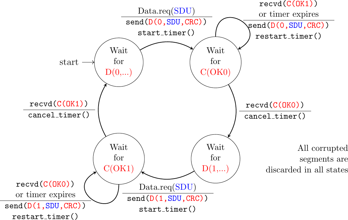
The initial state of the sender is Wait for D(0,…). In this state, the sender waits for a Data.request. The first data segment that it sends uses sequence number 0. After having sent this segment, the sender waits for an OK0 acknowledgment. A data segment is retransmitted upon expiration of the retransmission timer or if an acknowledgment with an incorrect sequence number has been received.

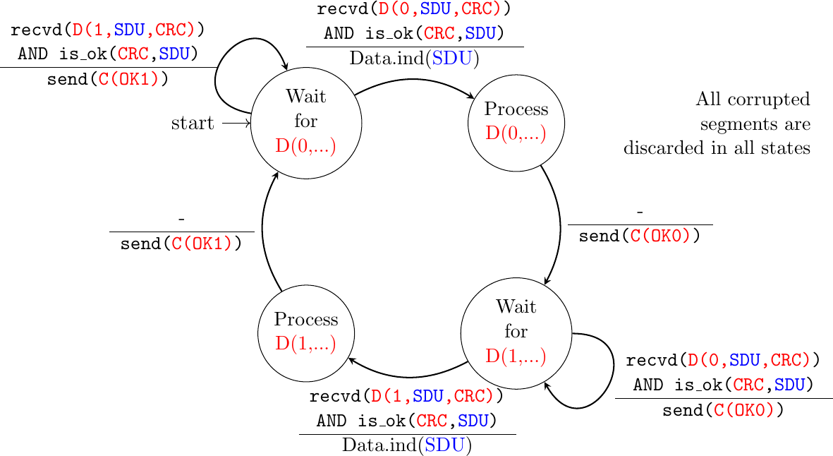
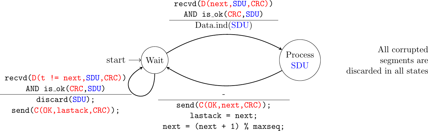
The receiver first waits for D(0,…). If the segment contains a correct CRC, it passes the SDU to its user and sends OK0. If the segment contains an invalid CRC, it is immediately discarded. Then, the receiver waits for D(1,…). In this state, it may receive a duplicate D(0,…) or a data segment with an invalid CRC. In both cases, it returns an OK0 segment to allow the sender to recover from the possible loss of the previous OK0 segment.

Fig. 49 Alternating bit protocol: Receiver FSM

Note

Corrupted segments must be discarded

The receiver FSM of the Alternating bit protocol discards all segments that contain an invalid CRC. This is the safest approach since the received segment can be completely different from the one sent by the remote host. A receiver should not attempt at extracting information from a corrupted segment because it cannot know which portion of the segment has been affected by the error.

The figure below illustrates the operation of the Alternating Bit Protocol.

The Alternating Bit Protocol can recover from the losses of data or control segments. This is illustrated in the two figures below. The first figure shows the loss of one data segment.

The second figure illustrates how the hosts handle the loss of one control segment.

The Alternating Bit Protocol can recover from transmission errors and segment losses. However, it has one important drawback. Consider two hosts that are directly connected by a 50 Kbits/sec satellite link that has a 250 milliseconds propagation delay. If these hosts send 1000 bits segments, then the maximum throughput that can be achieved by the alternating bit protocol is one segment every \(20+250+250=520\) milliseconds if we ignore the transmission time of the acknowledgment. This is less than 2 Kbits/sec !

Please log in to see this exercise

Please log in to see this exercise

Please log in to see this exercise

Go-back-n and selective repeat

To overcome the performance limitations of the alternating bit protocol, reliable protocols rely on pipelining shown in Fig. 50. This technique allows a sender to transmit several consecutive segments without being forced to wait for an acknowledgment after each segment. Each data segment contains a sequence number encoded as an n bits field.

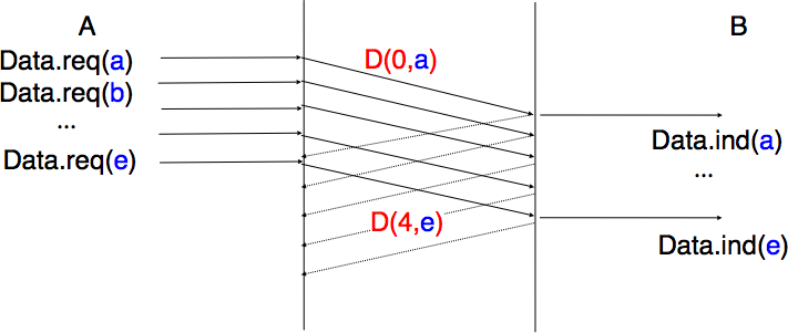
Fig. 50 Pipelining improves the performance of reliable protocols

Pipelining allows the sender to transmit segments at a higher rate. However this higher transmission rate may overload the receiver. In this case, the segments sent by the sender will not be correctly received by their final destination. The reliable protocols that rely on pipelining allow the sender to transmit W unacknowledged segments before being forced to wait for an acknowledgment from the receiving entity.

This is implemented by using a sliding window. The sliding window is the set of consecutive sequence numbers that the sender can use when transmitting segments without being forced to wait for an acknowledgment. Fig. 51 shows a sliding window containing five segments (6,7,8,9 and 10). Two of these sequence numbers (6 and 7) have been used to send segments and only three sequence numbers (8, 9 and 10) remain in the sliding window. The sliding window is said to be closed once all sequence numbers contained in the sliding window have been used.

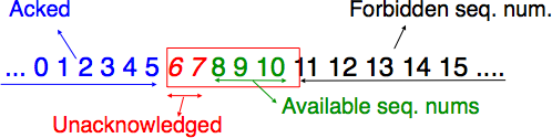
Fig. 51 The sliding window

Fig. 52 illustrates the operation of the sliding window. It uses a sliding window of three segments. The sender can thus transmit three segments before being forced to wait for an acknowledgment. The sliding window moves to the higher sequence numbers upon the reception of each acknowledgment. When the first acknowledgment (OK0) is received, it enables the sender to move its sliding window to the right and sequence number 3 becomes available. This sequence number is used later to transmit the segment containing d.

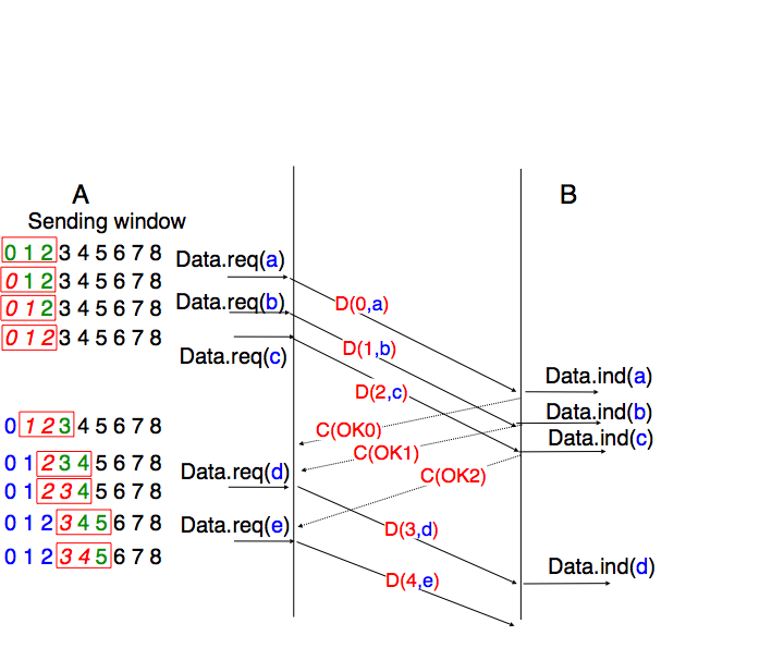
Fig. 52 Sliding window example

In practice, as the segment header includes an n bits field to encode the sequence number, only the sequence numbers between \(0\) and \(2^{n}-1\) can be used. This implies that, during a long transfer, the same sequence number will be used for different segments and the sliding window will wrap. This is illustrated in Fig. 53 assuming that 2 bits are used to encode the sequence number in the segment header. Note that upon reception of OK1, the sender slides its window and can use sequence number 0 again.

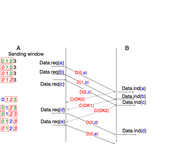
Fig. 53 Utilization of the sliding window with modulo arithmetic

Unfortunately, segment losses do not disappear because a reliable protocol uses a sliding window. To recover from losses, a sliding window protocol must define :

• a heuristic to detect losses

• a retransmission strategy to retransmit the lost segments

The simplest sliding window protocol uses the go-back-n recovery. Intuitively, go-back-n operates as follows. A go-back-n receiver is as simple as possible. It only accepts the segments that arrive in-sequence. A go-back-n receiver discards any out-of-sequence segment that it receives. When go-back-n receives a data segment, it always returns an acknowledgment containing the sequence number of the last in-sequence segment that it has received. This acknowledgment is said to be cumulative. When a go-back-n receiver sends an acknowledgment for sequence number x, it implicitly acknowledges the reception of all segments whose sequence number is earlier than x. A key advantage of these cumulative acknowledgments is that it is easy to recover from the loss of an acknowledgment. Consider for example a go-back-n receiver that received segments 1, 2 and 3. It sent OK1, OK2 and OK3. Unfortunately, OK1 and OK2 were lost. Thanks to the cumulative acknowledgments, when the sender receives OK3, it knows that all three segments have been correctly received.

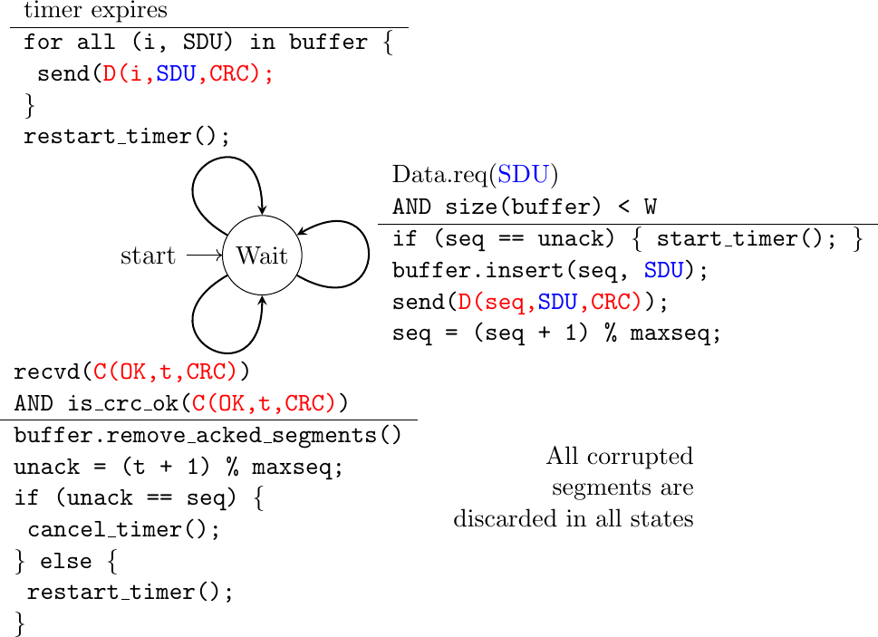
Fig. 54 shows the FSM of a simple go-back-n receiver. This receiver uses two variables : lastack and next. next is the next expected sequence number and lastack the sequence number of the last data segment that has been acknowledged. The receiver only accepts the segments that are received in sequence. maxseq is the number of different sequence numbers (\(2^n\)).

Fig. 54 Go-back-n: receiver FSM

A go-back-n sender is also very simple as shown in Fig. 55. It uses a sending buffer that can store an entire sliding window of segments [2]. The segments are sent with increasing sequence numbers (modulo maxseq). The sender must wait for an acknowledgment once its sending buffer is full. When a go-back-n sender receives an acknowledgment, it removes from the sending buffer all the acknowledged segments and uses a retransmission timer to detect segment losses. A simple go-back-n sender maintains one retransmission timer per connection. This timer is started when the first segment is sent. When the go-back-n sender receives an acknowledgment, it restarts the retransmission timer only if there are still unacknowledged segments in its sending buffer. When the retransmission timer expires, the go-back-n sender assumes that all the unacknowledged segments currently stored in its sending buffer have been lost. It thus retransmits all the unacknowledged segments in the buffer and restarts its retransmission timer.

Fig. 55 Go-back-n: sender FSM

The operation of go-back-n is illustrated in Fig. 56. In this figure, note that upon reception of the out-of-sequence segment D(2,c), the receiver returns a cumulative acknowledgment C(OK,0) that acknowledges all the segments that have been received in sequence. The lost segment is retransmitted upon the expiration of the retransmission timer.

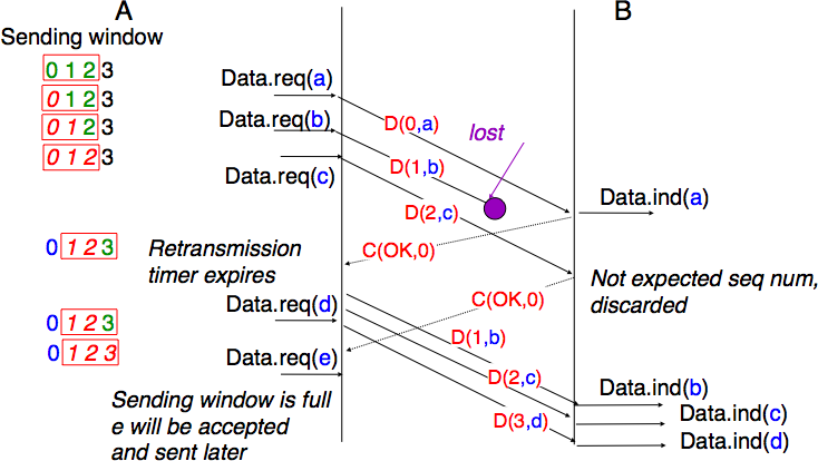
Fig. 56 Go-back-n : example

The main advantage of go-back-n is that it can be easily implemented, and it can also provide good performance when only a few segments are lost. However, when there are many losses, the performance of go-back-n quickly drops for two reasons :

• the go-back-n receiver does not accept out-of-sequence segments

• the go-back-n sender retransmits all unacknowledged segments once it has detected a loss

Please log in to see this exercise

Selective repeat is a better strategy to recover from losses. Intuitively, selective repeat allows the receiver to accept out-of-sequence segments. Furthermore, when a selective repeat sender detects losses, it only retransmits the segments that have been lost and not the segments that have already been correctly received.

A selective repeat receiver maintains a sliding window of W segments and stores in a buffer the out-of-sequence segments that it receives. Fig. 57 shows a five-segment receive window on a receiver that has already received segments 7 and 9.

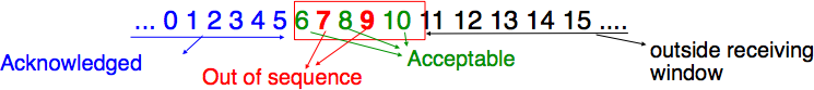
Fig. 57 The receiving window with selective repeat

A selective repeat receiver discards all segments having an invalid CRC, and maintains the variable lastack as the sequence number of the last in-sequence segment that it has received. The receiver always includes the value of lastack in the acknowledgments that it sends. Some protocols also allow the selective repeat receiver to acknowledge the out-of-sequence segments that it has received. This can be done for example by placing the list of the correctly received, but out-of-sequence segments in the acknowledgments together with the lastack value.

When a selective repeat receiver receives a data segment, it first verifies whether the segment is inside its receiving window. If yes, the segment is placed in the receive buffer. If not, the received segment is discarded and an acknowledgment containing lastack is sent to the sender. The receiver then removes all consecutive segments starting at lastack (if any) from the receive buffer. The payloads of these segments are delivered to the user, lastack and the receiving window are updated, and an acknowledgment acknowledging the last segment received in sequence is sent.

The selective repeat sender maintains a sending buffer that can store up to W unacknowledged segments. These segments are sent as long as the sending buffer is not full. Several implementations of a selective repeat sender are possible. A simple implementation associates one retransmission timer to each segment. The timer is started when the segment is sent and canceled upon reception of an acknowledgment that covers this segment. When a retransmission timer expires, the corresponding segment is retransmitted and this retransmission timer is restarted. When an acknowledgment is received, all the segments that are covered by this acknowledgment are removed from the sending buffer and the sliding window is updated.

Fig. 58 illustrates the operation of selective repeat when segments are lost. In this figure, C(OK,x) is used to indicate that all segments, up to and including sequence number x have been received correctly.

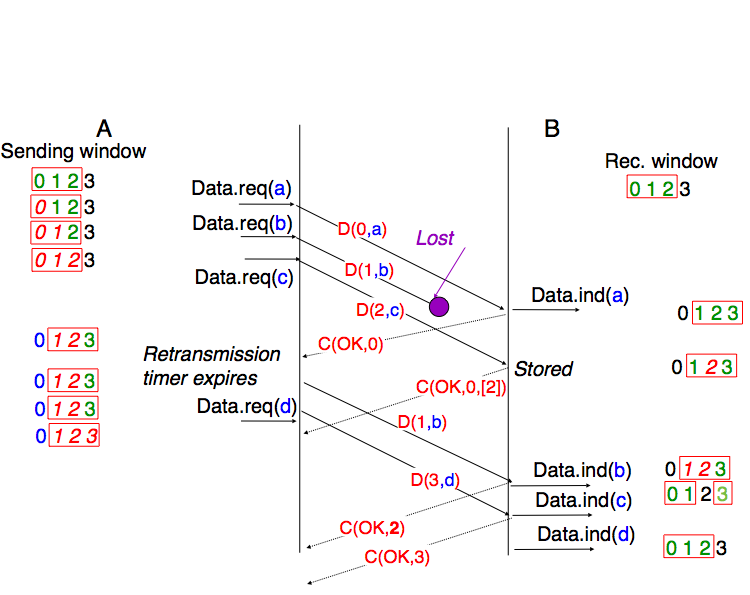
Fig. 58 Selective repeat : example

Pure cumulative acknowledgments work well with the go-back-n strategy. However, with only cumulative acknowledgments a selective repeat sender cannot easily determine which segments have been correctly received after a data segment has been lost. For example, in the figure above, the second C(OK,0) does not inform explicitly the sender of the reception of D(2,c) and the sender could retransmit this segment although it has already been received. A possible solution to improve the performance of selective repeat is to provide additional information about the received segments in the acknowledgments that are returned by the receiver. For example, the receiver could add in the returned acknowledgment the list of the sequence numbers of all segments that have already been received. Such acknowledgments are sometimes called selective acknowledgments. We will provide examples of such acknowledgments in the TCP and QUIC protocols later in this book.

Please log in to see this exercise

Note

Maximum window size with go-back-n and selective repeat

A reliable protocol that uses n bits to encode its sequence number can send up to \(2^n\) successive segments. However, to ensure a reliable delivery of the segments, go-back-n and selective repeat cannot use a sending window of \(2^n\) segments. Consider first go-back-n and assume that a sender sends \(2^n\) segments. These segments are received in-sequence by the destination, but all the returned acknowledgments are lost. The sender will retransmit all segments. These segments will all be accepted by the receiver and delivered a second time to the user. It is easy to see that this problem can be avoided if the maximum size of the sending window is \({2^n}-1\) segments. A similar problem occurs with selective repeat. However, as the receiver accepts out-of-sequence segments, a sending window of \({2^n}-1\) segments is not sufficient to ensure a reliable delivery. It can be easily shown that to avoid this problem, a selective repeat sender cannot use a window that is larger than \(\frac{2^n}{2}\) segments.

Reliable protocols often need to send data in both directions. To reduce the overhead caused by the acknowledgments, most reliable protocols use piggybacking. Thanks to this technique, an entity can place the acknowledgments and the receive window that it advertises for the opposite direction of the data flow inside the header of the data segments that it sends. The main advantage of piggybacking is that it reduces the overhead as it is not necessary to send a complete segment to carry an acknowledgment. This is illustrated in the figure below where the acknowledgment number is underlined in the data segments. Piggybacking is only used when data flows in both directions. A receiver will generate a pure acknowledgment when it does not send data in the opposite direction as shown in the bottom of the figure.

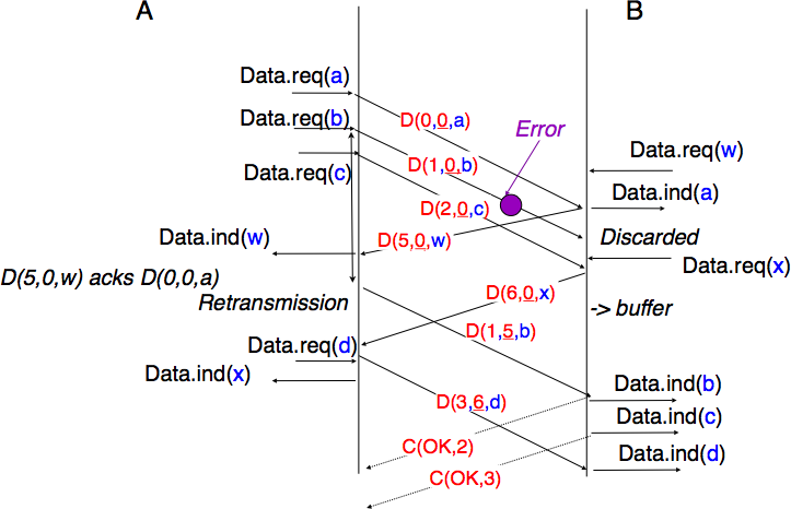
Fig. 59 Piggybacking example

Please log in to see this exercise

Please log in to see this exercise

Establishing a transport connection

Like the connectionless service, the connection-oriented service allows several applications running on a given host to exchange data with other hosts. The port numbers described earlier for the connectionless service are also used by the connection-oriented service to multiplex several applications. Similarly, connection-oriented protocols use checksums/CRCs to detect transmission errors and discard segments containing an invalid checksum/CRC.

An important difference between the connectionless service and the connection-oriented one is that the transport entities in the latter maintain some state during lifetime of the connection. This state is created when a connection is established and is removed when it is released.

The simplest approach to establish a transport connection would be to define two special control segments : CR (Connection Request) and CA (Connection Acknowledgment). The CR segment is sent by the transport entity that wishes to initiate a connection. If the remote entity wishes to accept the connection, it replies by sending a CA segment. The CR and CA segments contain port numbers that allow identifying the communicating applications. The transport connection is considered to be established once the CA segment has been received. At that point, data segments can be sent in both directions.

Unfortunately, this is not sufficient given the unreliability of the network layer. Since the network layer is imperfect, the CR or CA segments can be lost, delayed, or suffer from transmission errors. To deal with these problems, the control segments must be protected by a CRC or a checksum to detect transmission errors. Furthermore, since the CA segment acknowledges the reception of the CR segment, the CR segment should be protected using a retransmission timer.

Unfortunately, this scheme is not sufficient to ensure the reliability of the transport service. Consider for example a short-lived transport connection where a single, but important transfer (e.g. money transfer from a bank account) is sent. Such a short-lived connection starts with a CR segment acknowledged by a CA segment, then the data segment is sent, acknowledged and the connection terminates. Unfortunately, as the network layer service is unreliable, delays combined to retransmissions may lead to the situation depicted in the figure below, where a delayed CR and data segments from a former connection are accepted by the receiving entity as valid segments, and the corresponding data is delivered to the user. Duplicating SDUs is not acceptable, and the transport protocol must solve this problem.

To avoid these duplicates, transport protocols require the network layer to bound the Maximum Segment Lifetime (MSL). The organization of the network must guarantee that no segment remains in the network for longer than MSL seconds. For example, on today’s Internet, MSL is expected to be 2 minutes. To avoid duplicate transport connections, transport protocol entities must be able to safely distinguish between a duplicate CR segment and a new CR segment, without forcing each transport entity to remember all the transport connections that it has established in the past.

A classical solution to avoid remembering the previous transport connections to detect duplicates is to use a clock inside each transport entity. This transport clock has the following characteristics :

• the transport clock is implemented as a k bits counter and its clock cycle is such that \(2^k \times cycle >> MSL\). Furthermore, the transport clock counter is incremented every clock cycle and after each connection establishment. This clock is illustrated in Fig. 60.

• the transport clock must continue to be incremented even if the transport entity stops or reboots

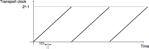
Fig. 60 Transport clock

It should be noted that transport clocks do not need and usually are not synchronized to the real-time clock. Precisely synchronizing real-time clocks is an interesting problem, but it is outside the scope of this document. See [Mills2006] for a detailed discussion on synchronizing the real-time clock.

This transport clock can be combined with an exchange of three segments, called the three way handshake, to detect duplicates. This three way handshake occurs as follows :

1. The initiating transport entity sends a CR segment. This segment requests the establishment of a transport connection. It contains a port number (not shown in the figure) and a sequence number (seq=x in the figure below) whose value is extracted from the transport clock. The transmission of the CR segment is protected by a retransmission timer.

2. The remote transport entity processes the CR segment and creates state for the connection attempt. At this stage, the remote entity does not yet know whether this is a new connection attempt or a duplicate segment. It returns a CA segment that contains an acknowledgment number to confirm the reception of the CR segment (ack=x in the figure below) and a sequence number (seq=y in the figure below) whose value is extracted from its transport clock. At this stage, the connection is not yet established.

3. The initiating entity receives the CA segment. The acknowledgment number of this segment confirms that the remote entity has correctly received the CR segment. The transport connection is considered to be established by the initiating entity and the numbering of the data segments starts at sequence number x. Before sending data segments, the initiating entity must acknowledge the received CA segments by sending another CA segment.

4. The remote entity considers the transport connection to be established after having received the segment that acknowledges its CA segment. The numbering of the data segments sent by the remote entity starts at sequence number y.

The three way handshake is illustrated in Fig. 61.

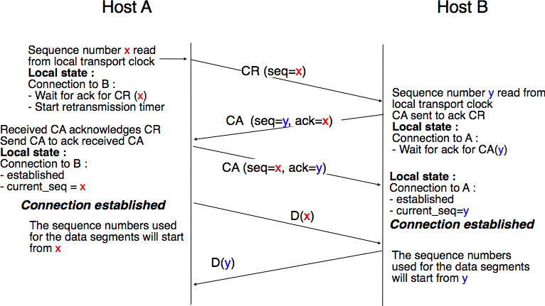
Fig. 61 The three-way handshake

Thanks to the three-way handshake, transport entities avoid duplicate transport connections. This is illustrated by considering the three scenarios below.

The first scenario (Fig. 62) is when the remote entity receives an old CR segment. It considers this CR segment as a connection establishment attempt and replies by sending a CA segment. However, the initiating host cannot match the received CA segment with a previous connection attempt. It sends a control segment (REJECT in the figure below) to cancel the spurious connection attempt. The remote entity cancels the connection attempt upon reception of this control segment.

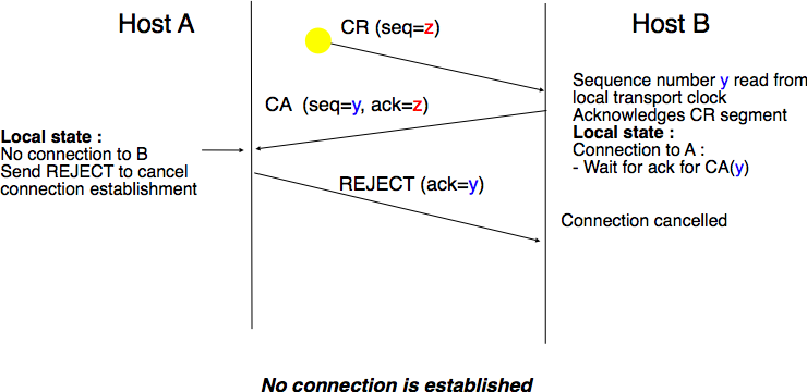
Fig. 62 Three-way handshake : recovery from a duplicate CR

A second scenario, shown in Fig. 63 is when the initiating entity sends a CR segment that does not reach the remote entity and receives a duplicate CA segment from a previous connection attempt. This duplicate CA segment cannot contain a valid acknowledgment for the CR segment as the sequence number of the CR segment was extracted from the transport clock of the initiating entity. The CA segment is thus rejected and the CR segment is retransmitted upon expiration of the retransmission timer.

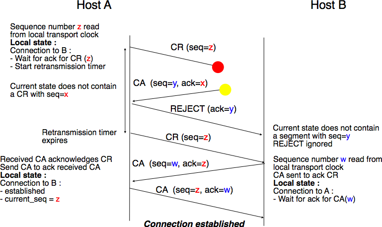
Fig. 63 Three-way handshake : recovery from a duplicate CA

The last scenario shown in Fig. 64 is less likely, but it is important to consider it as well. The remote entity receives an old CR segment. It notes the connection attempt and acknowledges it by sending a CA segment. The initiating entity does not have a matching connection attempt and replies by sending a REJECT. Unfortunately, this segment never reaches the remote entity. Instead, the remote entity receives a retransmission of an older CA segment that contains the same sequence number as the first CR segment. This CA segment cannot be accepted by the remote entity as a confirmation of the transport connection as its acknowledgment number cannot have the same value as the sequence number of the first CA segment.

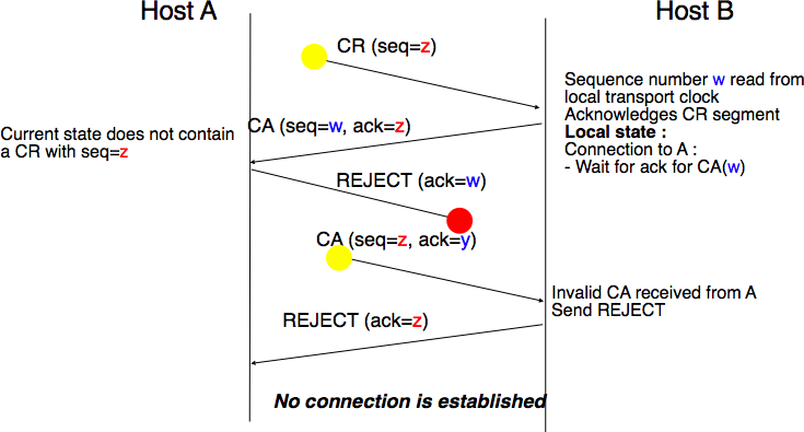
Fig. 64 Three-way handshake : recovery from duplicates CR and CA

Transferring data on a transport connection

Now that the transport connection has been established, it can be used to transfer data. To ensure a reliable delivery of the data, the transport protocol will include sliding windows, retransmission timers and go-back-n or selective repeat. However, we cannot simply reuse these techniques because a reliable transport protocol also needs to cope with three additional types of errors (i) variable delays, (ii) out-f-sequence delivery and (iii) segment duplication.

When two hosts are connected by a link, the transmission delay or the round-trip-time over the link is almost fixed. In a network that can span the globe, the delays and the round-trip-times can vary significantly on a per packet basis. This variability can be caused by two factors. First, packets sent through a network do not necessarily follow the same path to reach their destination. Second, some packets may be queued in the buffers of routers when the load is high and these queuing delays can lead to increased end-to-end delays.

Another problem is that a network does not always deliver packets in sequence. This implies that packets may be reordered by the network. Furthermore, the network may sometimes duplicate packets.

The last issue that needs to be dealt with in the transport layer is the transmission of large SDUs. In our example, we have used short SDUs which fit easily inside segments. Some applications generate SDUs that are much larger than the maximum size of a packet in the network layer. The transport layer needs to include mechanisms to fragment and reassemble these large SDUs.

To deal with all these characteristics of the network layer, we need to adapt the go-back-n and selective repeat techniques that we have introduced earlier.

The ability to detect transmission errors remains important. Each segment contains a CRC/checksum which is computed over the entire segment (header and payload) by the sender and inserted in the header. The receiver recomputes the CRC/checksum for each received segment and discards all segments with an invalid CRC.

Reliable transport protocols also use sequence numbers and acknowledgment numbers. While our example protocols used one sequence number per segment, some reliable transport protocols consider all the data transmitted as a stream of bytes. In these protocols, the sequence number placed in the segment header corresponds to the position of the first byte of the payload in the bytestream. This sequence number allows detecting losses but also enables the receiver to reorder the out-of-sequence segments. This is illustrated in the figure below.

Using sequence numbers to count bytes has also one advantage when the transport layer needs to fragment SDUs in several segments. The figure below shows the fragmentation of a large SDU in two segments. Upon reception of the segments, the receiver will use the sequence numbers to correctly reorder the data.

Compared to our simple protocols, reliable transport protocols encode their sequence numbers using more bits. 32 bits and 64 bits sequence numbers are frequent in the transport layer. This large sequence number space is motivated by two reasons. First, since the sequence number is incremented for each transmitted byte, a single segment may consume one or several thousands of sequence numbers. Second, a reliable transport protocol must be able to detect delayed segments. This can only be done if the number of bytes transmitted during the MSL period is smaller than the sequence number space. Otherwise, there is a risk of accepting duplicate segments.

Go-back-n and selective repeat can be used in the transport layer as in the datalink layer. Since the network layer does not guarantee an in-order delivery of the packets, a transport entity should always store the segments that it receives out-of-sequence. For this reason, most transport protocols will opt for some form of selective repeat mechanism.

In simple protocols, the sliding window has usually a fixed size which depends on the amount of available buffers. A single transport layer entity serves a large and varying number of application processes. Each transport layer entity manages a pool of buffers that needs to be shared between all these processes. Transport entity are usually implemented inside the operating system kernel and shares memory with other parts of the system. Furthermore, a transport layer entity must support several (possibly hundreds or thousands) of transport connections at the same time. This implies that the memory which can be used to support the sending or the receiving buffer of a transport connection may change during the lifetime of the connection [3] . Thus, a transport protocol must allow the sender and the receiver to adjust their window sizes.

To deal with this issue, transport protocols allow the receiver to advertise the current size of its receiving window in all the acknowledgments that it sends. The receiving window advertised by the receiver bounds the size of the sending buffer used by the sender. In practice, the sender maintains two state variables : swin, the size of its sending window (that may be adjusted by the system) and rwin, the size of the receiving window advertised by the receiver. At any time, the number of unacknowledged segments cannot be larger than \(\min(swin,rwin)\) [4] . The utilization of dynamic windows is illustrated in figure Fig. 65.

Fig. 65 Dynamic receiving window

The receiver may adjust its advertised receive window based on its current memory consumption, but also to limit the bandwidth used by the sender. In practice, the receive buffer can also shrink as the application may not able to process the received data quickly enough. In this case, the receive buffer may be completely full and the advertised receive window may shrink to 0. When the sender receives an acknowledgment with a receive window set to 0, it is blocked until it receives an acknowledgment with a positive receive window. Unfortunately, as shown in Fig. 66, the loss of this acknowledgment could cause a deadlock as the sender waits for an acknowledgment while the receiver is waiting for a data segment.

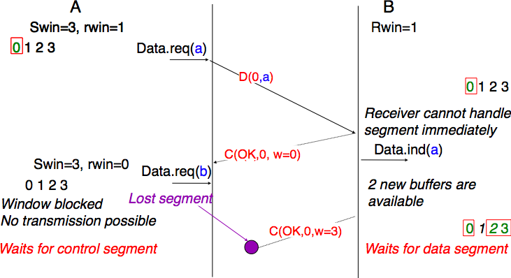
Fig. 66 Risk of deadlock with dynamic windows

To solve this problem, transport protocols rely on a special timer : the persistence timer. This timer is started by the sender whenever it receives an acknowledgment advertising a receive window set to 0. When the timer expires, the sender retransmits an old segment in order to force the receiver to send a new acknowledgment, and hence send the current receive window size.

To conclude our description of the basic mechanisms found in transport protocols, we still need to discuss the impact of segments arriving in the wrong order. If two consecutive segments are reordered, the receiver relies on their sequence numbers to reorder them in its receive buffer. Unfortunately, as transport protocols reuse the same sequence number for different segments, if a segment is delayed for a prolonged period of time, it might still be accepted by the receiver. This is illustrated in Fig. 67 where segment D(1,b) is delayed.

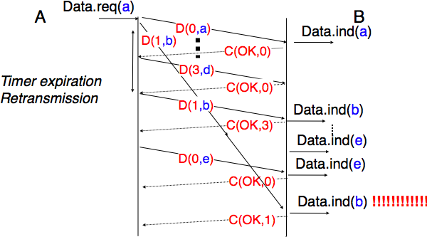
Fig. 67 Ambiguities caused by excessive delays

To deal with this problem, transport protocols combine two solutions. First, they use 32 bits or more to encode the sequence number in the segment header. This increases the overhead, but also increases the delay between the transmission of two different segments having the same sequence number. Second, transport protocols require the network layer to enforce a Maximum Segment Lifetime (MSL). The network layer must ensure that no packet remains in the network for more than MSL seconds. In the Internet the MSL is assumed [5] to be 2 minutes RFC 793. Note that this limits the maximum bandwidth of a transport protocol. If it uses n bits to encode its sequence numbers, then it cannot send more than \(2^n\) segments every MSL seconds.

Closing a transport connection

When we discussed the connection-oriented service, we mentioned that there are two types of connection releases : abrupt release and graceful release.

The first solution to release a transport connection is to define a new control segment (e.g. the DR segment for Disconnection Request) and consider the connection to be released once this segment has been sent or received. This is illustrated in Fig. 68.

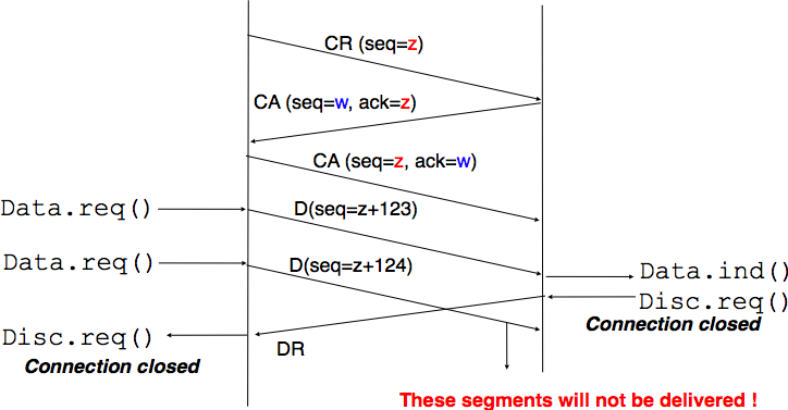
Fig. 68 Abrupt connection release

As the entity that sends the DR segment cannot know whether the other entity has already sent all its data on the connection, SDUs can be lost during such an abrupt connection release.

The second method to release a transport connection is to release independently the two directions of data transfer. Once a user of the transport service has sent all its SDUs, it performs a DISCONNECT.req for its direction of data transfer. The transport entity sends a control segment to request the release of the connection after the delivery of all previous SDUs to the remote user. This is usually done by placing in the DR the next sequence number and by delivering the DISCONNECT.ind only after all previous DATA.ind. The remote entity confirms the reception of the DR segment and the release of the corresponding direction of data transfer by returning an acknowledgment. This is illustrated in Fig. 69.

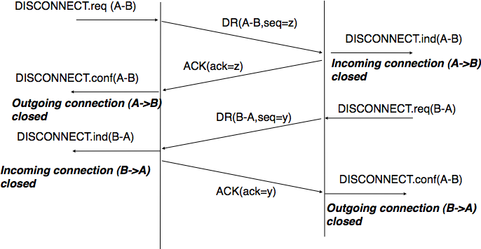
Fig. 69 Graceful connection release

Footnotes

[1]

SDU is the acronym of Service Data Unit. We use it as a generic term to represent the data that is transported by a protocol.

[2]

The size of the sliding window can be either fixed for a given protocol or negotiated during the connection establishment phase. Some protocols allow to change the maximum window size during the data transfer. We will explain these techniques with real protocols later.

[3]

For a discussion on how the sending buffer can change, see e.g. [SMM1998]

[4]

Note that if the receive window shrinks, it might happen that the sender has already sent a segment that is not anymore inside its window. This segment will be discarded by the receiver and the sender will retransmit it later.

[5]

In reality, the Internet does not strictly enforce this MSL. However, it is reasonable to expect that most packets on the Internet will not remain in the network during more than 2 minutes. There are a few exceptions to this rule, such as RFC 1149 whose implementation is described in http://www.blug.linux.no/rfc1149/ but there are few real links supporting RFC 1149 in the Internet.