Introduction

The first step when building a network, even a worldwide network such as the Internet, is to connect two hosts together. This is illustrated in figure Fig. 1.

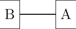
Fig. 1 Connecting two hosts together

To enable the two hosts to exchange information, they need to be linked together by some kind of physical media. Computer networks have used various types of physical media to exchange information, notably :

• electrical cable. Information can be transmitted over different types of electrical cables. The most common ones are the twisted pairs (that are used in the telephone network, but also in enterprise networks) and the coaxial cables (that are still used in cable TV networks, but are no longer used in enterprise networks). Some networking technologies operate over the classical electrical cable.

• Optical fiber. Optical fibers are frequently used in public and enterprise networks when the distance between the communication devices is larger than one kilometer. There are two main types of optical fibers : multi-mode and single-mode. Multi-mode is much cheaper than single-mode fiber because a LED can be used to send a signal over a multi-mode fiber while a single-mode fiber must be driven by a laser. Due to the different modes of propagation of light, multi-mode fibers are limited to distances of a few kilometers while single-mode fibers can be used over distances greater than several tens of kilometers. In both cases, repeaters can be used to regenerate the optical signal at one endpoint of a fiber to send it over another fiber.

• Wireless. In this case, a radio signal is used to encode the information exchanged between the communicating devices. Many types of modulation techniques are used to send information over a wireless channel and there is a lot of innovation in this field with new techniques appearing every year. While most wireless networks rely on radio signals, some use a laser that sends light pulses to a remote detector. These optical techniques allow us to create point-to-point links while radio-based techniques can be used to build networks containing devices spread over a small geographical area.

The physical layer

These physical media can be used to exchange information once this information has been converted into a suitable electrical signal. Entire telecommunication courses and textbooks are devoted to the problem of converting analog or digital information into an electrical signal so that it can be transmitted over a given physical link. In this book, we only consider two very simple schemes that allow us to transmit information over an electrical cable. This enables us to highlight the key problems when transmitting information over a physical link. We are only interested in techniques that allow transmitting digital information through the wire. Here, we will focus on the transmission of bits, i.e. either 0 or 1.

Note

Bit rate

In computer networks, the bit rate of the physical layer is always expressed in bits per second. One Mbps is one million bits per second, and one Gbps is one billion bits per second. This is in contrast with memory specifications that are usually expressed in bytes (8 bits), KiloBytes (1024 bytes), or MegaBytes (1048576 bytes). Transferring one MByte through a 1 Mbps link lasts 8.39 seconds.

Bit rate	Bits per second
1 Kbps	\(10^3\)
1 Mbps	\(10^6\)
1 Gbps	\(10^9\)
1 Tbps	\(10^{12}\)

To understand some of the principles behind the physical transmission of information, let us consider the simple case of an electrical wire that is used to transmit bits. Assume that the two communicating hosts want to transmit one thousand bits per second. To transmit these bits, the two hosts can agree on the following rules :

• On the sender side :

  • set the voltage on the electrical wire at +5V during one millisecond to transmit a bit set to 1

  • set the voltage on the electrical wire at -5V during one millisecond to transmit a bit set to 0

• On the receiver side :

  • every millisecond, record the voltage applied on the electrical wire. If the voltage is set to +5V, record the reception of bit 1. Otherwise, record the reception of bit 0

This transmission scheme has been used in some early networks. We use it as a basis to understand how hosts communicate. From a computer science viewpoint, dealing with voltages is unusual. Computer scientists frequently rely on models that enable them to reason about the issues that they face without having to consider all implementation details. The physical transmission scheme described above can be represented by using a time-sequence diagram.

A time-sequence diagram describes the interactions between communicating hosts. By convention, the communicating hosts are represented in the left and right parts of the diagram, while the electrical link occupies the middle of the diagram. In such a time-sequence diagram, time flows from the top to the bottom of the diagram. The transmission of one bit of information is represented by three arrows. Starting from the left, the first horizontal arrow represents the request to transmit one bit of information. This request is represented by a primitive, which can be considered as a kind of procedure call. This primitive has one parameter (the bit being transmitted) and a name (DATA.request in this example). By convention, all primitives that are named something.request correspond to a request to transmit some information. The dashed arrow indicates the transmission of the corresponding electrical signal on the wire. Electrical and optical signals do not travel instantaneously. The diagonal dashed arrow indicates that it takes some time for the electrical signal to be transmitted from Host A to Host B. Upon reception of the electrical signal, the electronics on Host B’s network interface detect the voltage and convert it into a bit. This bit is delivered as a DATA.indication primitive. All primitives that are named something.indication correspond to the reception of some information. The dashed lines also represent the relationship between two (or more) primitives. Such a time-sequence diagram provides information about the ordering of the different primitives, but the distance between two primitives does not represent a precise amount of time.

Time-sequence diagrams are useful when trying to understand the characteristics of a given communication scheme. When considering the above transmission scheme, it is useful to evaluate whether this scheme allows the two communicating hosts to reliably exchange information. A digital transmission is considered reliable when a sequence of bits that is transmitted by a host is received correctly at the other end of the wire. In practice, achieving perfect reliability when transmitting information using the above scheme is difficult. Several problems can occur with such a transmission scheme.

The first problem is that electrical transmission can be affected by electromagnetic interference. Interference can have various sources including natural phenomena (like thunderstorms, variations of the magnetic field,…) but also other electrical signals (such as interference from neighboring cables, interference from neighboring antennas,…). Due to these various types of interference, there is unfortunately no guarantee that when a host transmits one bit on a wire, the same bit is received at the other end. This is illustrated in the figure below where a DATA.request(0) on the left host leads to a Data.indication(1) on the right host.

With the above transmission scheme, a bit is transmitted by setting the voltage on the electrical cable to a specific value during some period of time. We have seen that due to electromagnetic interference, the voltage measured by the receiver can differ from the voltage set by the transmitter. This is the main cause of transmission errors. However, this is not the only type of problem that can occur. Besides defining the voltages for bits 0 and 1, the above transmission scheme also specifies the duration of each bit. If one million bits are sent every second, then each bit lasts 1 microsecond. On each host, the transmission (resp. the reception) of each bit is triggered by a local clock having a 1 MHz frequency. These clocks are the second source of problems when transmitting bits over a wire. Although the two clocks have the same specification, they run on different hosts, possibly at a different temperature and with a different source of energy. In practice, it is possible that the two clocks do not operate at exactly the same frequency. Assume that the clock of the transmitting host operates at exactly 1000000 Hz while the receiving clock operates at 999999 Hz. This is a very small difference between the two clocks. However, when using the clock to transmit bits, this difference is important. With its 1000000 Hz clock, the transmitting host will generate one million bits during a period of one second. During the same period, the receiving host will sense the wire 999999 times and thus will receive one bit less than the bits originally transmitted. This small difference in clock frequencies implies that bits can “disappear” during their transmission on an electrical cable. This is illustrated in the figure below.

A similar reasoning applies when the clock of the sending host is slower than the clock of the receiving host. In this case, the receiver will sense more bits than the bits that have been transmitted by the sender. This is illustrated in the figure below where the second bit received on the right was not transmitted by the left host.

From a Computer Science viewpoint, the physical transmission of information through a wire is often considered as a black box that allows transmitting bits. This black box is commonly referred to as the physical layer service and is represented by using the DATA.request and DATA.indication primitives introduced earlier. This physical layer service facilitates the sending and receiving of bits, by abstracting the technological details that are involved in the actual transmission of the bits as an electromagnetic signal. However, it is important to remember that the physical layer service is imperfect and has the following characteristics :

• the Physical layer service may change, e.g. due to electromagnetic interference, the value of a bit being transmitted

• the Physical layer service may deliver more bits to the receiver than the bits sent by the sender

• the Physical layer service may deliver fewer bits to the receiver than the bits sent by the sender.

Many other types of encodings have been defined to transmit information over an electrical cable. All physical layers are able to send and receive physical symbols that represent values 0 and 1. However, for various reasons that are outside the scope of this chapter, several physical layers exchange other physical symbols as well. For example, the Manchester encoding used in several physical layers can send four different symbols. The Manchester encoding is a differential encoding scheme in which time is divided into fixed-length periods. Each period is divided into two halves and two different voltage levels can be applied. To send a symbol, the sender must set one of these two voltage levels during each half period. To send a 1 (resp. 0), the sender must set a high (resp. low) voltage during the first half of the period and a low (resp. high) voltage during the second half. This encoding ensures that there will be a transition at the middle of each period and allows the receiver to synchronize its clock to the sender’s clock. Apart from the encodings for 0 and 1, the Manchester encoding also supports two additional symbols : InvH and InvB where the same voltage level is used for the two half periods. By definition, these two symbols cannot appear inside a frame which is only composed of 0 and 1. Some technologies use these special symbols as markers for the beginning or end of frames. This encoding is illustrated in Fig. 2.

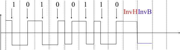
Fig. 2 Manchester encoding

When the physical layer transmits a bit of information using light or an electromagnetic signal, there is no guarantee that the bit sent by the transmitter will be received as it was sent by the receiver. Several types of errors can impact this transmission.

Information Theory defines two mechanisms that can be used to transmit information over a channel affected by random errors. These two mechanisms add redundancy to the transmitted information, to allow the receiver to detect or sometimes even correct transmission errors. A detailed discussion of these mechanisms is outside the scope of this chapter, but it is useful to consider a simple mechanism to understand its operation and its limitations.

Information theory defines coding schemes. There are different types of coding schemes, but let us focus on coding schemes that operate on binary strings. A coding scheme is a function that maps information encoded as a string of m bits into a string of n bits. The simplest coding scheme is the (even) parity coding. This coding scheme takes an m bits source string and produces an m+1 bits coded string where the first m bits of the coded string are the bits of the source string and the last bit of the coded string is chosen such that the coded string will always contain an even number of bits set to 1. For example :

• 1001 is encoded as 10010

• 1101 is encoded as 11011

This parity scheme has been used in some RAMs as well as to encode characters sent over a serial line. It is easy to show that this coding scheme allows the receiver to detect a single transmission error, but it cannot correct it. However, if two or more bits are in error, the receiver may not always be able to detect the error.

Some coding schemes allow the receiver to correct some transmission errors. For example, consider the coding scheme that encodes each source bit as follows :

• 1 is encoded as 111

• 0 is encoded as 000

For example, consider a sender that sends 111. If there is one bit in error, the receiver could receive 011 or 101 or 110. In these three cases, the receiver will decode the received bit pattern as a 1 since it contains a majority of bits set to 1. If there are two bits in error, the receiver will not be able anymore to recover from the transmission error.

This simple coding scheme forces the sender to transmit three bits for each source bit. However, it allows the receiver to correct single bit errors. More advanced coding systems that allow recovering from errors are used in several types of physical layers.

To understand error detection codes, let us consider two devices that exchange bit strings containing N bits. To allow the receiver to detect a transmission error, the sender converts each string of N bits into a string of N+r bits. Usually, the r redundant bits are added at the beginning or the end of the transmitted bit string, but some techniques interleave redundant bits with the original bits. An error detection code can be defined as a function that computes the r redundant bits corresponding to each string of N bits. The simplest error detection code is the parity bit. There are two types of parity schemes : even and odd parity. With the even (resp. odd) parity scheme, the redundant bit is chosen so that an even (resp. odd) number of bits are set to 1 in the transmitted bit string of N+r bits. The receiver can easily recompute the parity of each received bit string and discard the strings with an invalid parity. The parity scheme is often used when 7-bit characters are exchanged. In this case, the eighth bit is often a parity bit. The table below shows the parity bits that are computed for bit strings containing three bits.

3 bits string	Odd parity	Even parity
000	1	0
001	0	1
010	0	1
100	0	1
111	0	1
110	1	0
101	1	0
011	1	0

The parity bit allows a receiver to detect transmission errors that have affected a single bit among the transmitted N+r bits. If there are two or more bits in error, the receiver may not necessarily be able to detect the transmission error. More powerful error detection schemes have been defined. The Cyclical Redundancy Checks (CRC) are widely used in datalink layer protocols. An N-bits CRC can detect all transmission errors affecting a burst of less than N bits in the transmitted frame and all transmission errors that affect an odd number of bits. Additional details about CRCs may be found in [Williams1993].

It is also possible to design a code that allows the receiver to correct transmission errors. The simplest error correction code is the triple modular redundancy (TMR). To transmit a bit set to 1 (resp. 0), the sender transmits 111 (resp. 000). When there are no transmission errors, the receiver can decode 111 as 1. If transmission errors have affected a single bit, the receiver performs majority voting as shown in the table below. This scheme allows the receiver to correct all transmission errors that affect a single bit.

Received bits	Decoded bit
000	0
001	0
010	0
100	0
111	1
110	1
101	1
011	1

Other more powerful error correction codes have been proposed and are used in some applications. The Hamming Code is a clever combination of parity bits that provides error detection and correction capabilities.

All the functions related to the physical transmission or information through a wire (or a wireless link) are usually known as the physical layer. The physical layer allows two or more entities that are directly attached to the same transmission medium to exchange bits. Being able to exchange bits is important as virtually any information can be encoded as a sequence of bits. Electrical engineers are used to processing streams of bits, but computer scientists usually prefer to deal with higher-level concepts.

A similar issue arises with file storage. Storage devices such as hard-disks also store streams of bits. There are hardware devices that process the bit stream produced by a hard-disk, but computer scientists have designed filesystems to allow applications to easily access such storage devices. These filesystems are typically divided into several layers as well. Hard-disks store sectors of 512 bytes or more. Unix filesystems group sectors in larger blocks that can contain data or inodes representing the structure of the filesystem. Finally, applications manipulate files and directories that are translated into blocks, sectors, and eventually bits by the operating system.

Computer networks use a similar approach. Each layer provides a service that is built above the underlying layer and is closer to the needs of the applications. Fig. 3 represents the lower layer of the protocol stack. We will explore the different layers of this stack in this book.

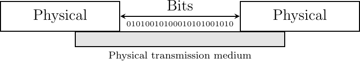
Fig. 3 The Physical layer

The datalink layer

Computer scientists are usually not interested in exchanging bits between two hosts. They prefer to write software that deals with larger blocks of data in order to transmit messages or complete files. Thanks to the physical layer service, it is possible to send a continuous stream of bits between two hosts. This stream of bits can include logical blocks of data, but we need to be able to extract each block of data from the bit stream despite the imperfections of the physical layer. In many networks, the basic unit of information exchanged between two directly connected hosts is often called a frame. A frame can be defined as a sequence of bits that has a particular syntax or structure. We will see examples of such frames later in this chapter.

To enable the transmission/reception of frames, the first problem to be solved is how to encode a frame as a sequence of bits, so that the receiver can easily recover the received frame despite the limitations of the physical layer.

If the physical layer were perfect, the problem would be very simple. We would simply need to define how to encode each frame as a sequence of consecutive bits. The receiver would then easily be able to extract the frames from the received bits. Unfortunately, the imperfections of the physical layer make this framing problem slightly more complex. Several solutions have been proposed and are used in practice in different network technologies.

Framing

The framing problem can be defined as : “How does a sender encode frames so that the receiver can efficiently extract them from the stream of bits that it receives from the physical layer”.

A first solution to this problem is to require the physical layer to remain idle for some time after the transmission of each frame. These idle periods can be detected by the receiver and serve as a marker to delineate frame boundaries. Unfortunately, this solution is not acceptable for two reasons. First, some physical layers cannot remain idle and always need to transmit bits. Second, inserting an idle period between frames decreases the maximum bit rate that can be achieved.

Note

Bit rate and bandwidth

Bit rate and bandwidth are often used to characterize the transmission capacity of the physical service. The original definition of bandwidth, as listed in the Webster dictionary is a range of radio frequencies which is occupied by a modulated carrier wave, which is assigned to a service, or over which a device can operate. This definition corresponds to the characteristics of a given transmission medium or receiver. For example, the human ear is able to decode sounds in roughly the 0-20 KHz frequency range. By extension, bandwidth is also used to represent the capacity of a communication system in bits per second. For example, a Gigabit Ethernet link is theoretically capable of transporting one billion bits per second.

Given that multi-symbol encodings cannot be used by all physical layers, a generic solution which can be used with any physical layer that is able to transmit and receive only bits 0 and 1 is required. This generic solution is called stuffing and two variants exist : bit stuffing and character stuffing. To enable a receiver to easily delineate the frame boundaries, these two techniques reserve special bit strings as frame boundary markers and encode the frames so that these special bit strings do not appear inside the frames.

Bit stuffing reserves the 01111110 bit string as the frame boundary marker and ensures that there will never be six consecutive 1 symbols transmitted by the physical layer inside a frame. With bit stuffing, a frame is sent as follows. First, the sender transmits the marker, i.e. 01111110. Then, it sends all the bits of the frame and inserts an additional bit set to 0 after each sequence of five consecutive 1 bits. This ensures that the sent frame never contains a sequence of six consecutive bits set to 1. As a consequence, the marker pattern cannot appear inside the frame sent. The marker is also sent to mark the end of the frame. The receiver performs the opposite to decode a received frame. It first detects the beginning of the frame thanks to the 01111110 marker. Then, it processes the received bits and counts the number of consecutive bits set to 1. If a 0 follows five consecutive bits set to 1, this bit is removed since it was inserted by the sender. If a 1 follows five consecutive bits set to 1, it indicates a marker if it is followed by a bit set to 0. The table below illustrates the application of bit stuffing to some frames.

Original frame	Transmitted frame
0001001001001001001000011	01111110000100100100100100100001101111110
0110111111111111111110010	01111110011011111011111011111011001001111110
0111110	011111100111110001111110
01111110	0111111001111101001111110

For example, consider the transmission of 0110111111111111111110010. The sender will first send the 01111110 marker followed by 011011111. After these five consecutive bits set to 1, it inserts a bit set to 0 followed by 11111. A new 0 is inserted, followed by 11111. A new 0 is inserted followed by the end of the frame 110010 and the 01111110 marker.

Bit stuffing increases the number of bits required to transmit each frame. The worst case for bit stuffing is of course a long sequence of bits set to 1 inside the frame. If transmission errors occur, stuffed bits or markers can be in error. In these cases, the frame affected by the error and possibly the next frame will not be correctly decoded by the receiver, but it will be able to resynchronize itself at the next valid marker.

Bit stuffing can be easily implemented in hardware. However, implementing it in software is difficult given the complexity of performing bit manipulations in software. Software implementations prefer to process characters than bits; software-based datalink layers usually use character stuffing. This technique operates on frames that contain an integer number of characters. In computer networks, characters are usually encoded by relying on the ASCII table. This table defines the encoding of various alphanumeric characters as a sequence of bits. RFC 20 provides the ASCII table that is used by many Internet protocols. For example, the table defines the following binary representations :

• A : 1000011 b

• 0 : 0110000 b

• z : 1111010 b

• @ : 1000000 b

• space : 0100000 b

In addition, the ASCII table also defines several non-printable or control characters. These characters were designed to allow an application to control a printer or a terminal. These control characters include CR and LF, that are used to terminate a line, and the BEL character which causes the terminal to emit a sound.

• NUL: 0000000 b

• BEL: 0000111 b

• CR : 0001101 b

• LF : 0001010 b

• DLE: 0010000 b

• STX: 0000010 b

• ETX: 0000011 b

Some characters are used as markers to delineate the frame boundaries. Many character stuffing techniques use the DLE, STX, and ETX characters of the ASCII character set. DLE STX (resp. DLE ETX) is used to mark the beginning (end) of a frame. When transmitting a frame, the sender adds a DLE character after each transmitted DLE character. This ensures that none of the markers can appear inside the transmitted frame. The receiver detects the frame boundaries and removes the second DLE when it receives two consecutive DLE characters. For example, to transmit frame 1 2 3 DLE STX 4, a sender will first send DLE STX as a marker, followed by 1 2 3 DLE. Then, the sender transmits an additional DLE character followed by STX 4 and the DLE ETX marker.

Original frame	Transmitted frame
1 2 3 4	DLE STX 1 2 3 4 DLE ETX
1 2 3 DLE STX 4	DLE STX 1 2 3 DLE DLE STX 4 DLE ETX
DLE STX DLE ETX	DLE STX DLE DLE STX DLE DLE ETX DLE ETX

Character stuffing, like bit stuffing, increases the length of the transmitted frames. For character stuffing, the worst frame is a frame containing many DLE characters. When transmission errors occur, the receiver may incorrectly decode one or two frames (e.g. if the errors occur in the markers). However, it will be able to resynchronize itself with the next correctly received markers.

Bit stuffing and character stuffing allow recovering frames from a stream of bits or bytes. This framing mechanism provides a richer service than the physical layer. Through the framing service, one can send and receive complete frames. This framing service can also be represented by using the DATA.request and DATA.indication primitives. This is illustrated in the figure below, assuming hypothetical frames containing four useful bits and one bit of framing for graphical reasons.

We can now build upon the framing mechanism to allow the hosts to exchange frames containing an integer number of bits or bytes. Once the framing problem has been solved, we can use these frames to carry Internet packets.

Coping with transmission errors

As explained earlier, the physical layer can be subject to various types that affect the bits sent by a transmitter. Data transmission on a physical link can be affected by the following errors :

• random isolated errors where the value of a single bit has been modified due to a transmission error

• random burst errors where the values of n consecutive bits have been changed due to transmission errors

• random bit creations and random bit removals where bits have been added or removed due to transmission errors

Besides framing, datalink layers also include mechanisms to detect and sometimes even recover from transmission errors. To allow a receiver to notice transmission errors, a sender must add some redundant information as an error detection code to the frame sent. This error detection code is computed by the sender on the frame that it transmits. When the receiver receives a frame with an error detection code, it recomputes it and verifies whether the received error detection code matches the computed error detection code. If they match, the frame is considered to be valid.

Please log in to see this exercise

Please log in to see this exercise

Note

Framing on the Internet

The bit stuffing and character stuffing described above are generic solutions applied by various protocols. When Internet hosts used dial-up modems or serial transmission to exchange data, they used protocols such as SLIP defined in RFC 1035 or PPP defined in RFC 1661.

The Serial Line IP (SLIP) protocol uses character stuffing with two special characters (END, 192 in decimal and ESC, 219 in decimal).

The Point-to-Point Protocol (PPP) supports different techniques of framing. RFC 1662 describes how character stuffing and bit stuffing can be used by PPP.

Fig. 126 illustrates the second layer of the protocol stack that uses the services provided by the Physical layer to exchange frames. We will use the word frame throughout this book to refer to the unit of information exchanged between two datalink layer entities.

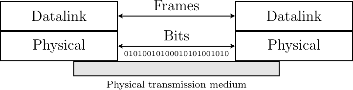
Fig. 4 The Datalink layer in the protocol stack

The network layer

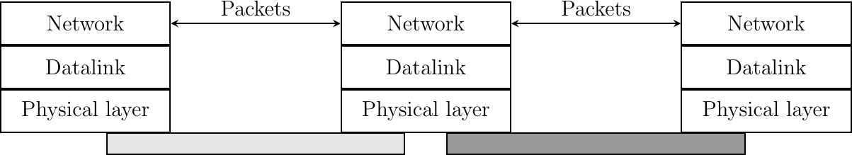
The Datalink layer allows directly connected hosts to exchange information, but it is often necessary to exchange information between hosts that are not attached to the same physical medium. This is the task of the network layer. The network layer is built above the datalink layer. Network layer entities exchange packets. A packet is a finite sequence of bytes that is transported by the datalink layer inside one or more frames. A packet usually contains information about its origin and its destination, and usually passes through several intermediate devices called routers on its way from its origin to its destination. This is illustrated in Fig. 5.

Fig. 5 The network layer

Internet hosts such as laptops, smartphones, PCs, servers, and various Internet of Things (IoT) devices connect to the Internet through various types of datalink layer technologies. Popular datalink layer technologies include Wi-Fi, Ethernet, Bluetooth, and the different types of cellular network technologies such as 4G and 5G. Some of these technologies will be discussed in the second part of this book. They have very specific characteristics that we ignore in this part of the book.

The Internet relies on a few architectural principles. First, all the information that hosts exchange must be divided into IP packets. IP stands for the Internet Protocol. This is the protocol or the set of rules that hosts apply when exchanging information. An IP packet is a variable-length sequence of bytes that contains two main parts :

• a header which contains control information specifying notably the source and the destination of the payload

• a payload which contains the data to be exchanged

A second principle is that each host is identified by a unique IP address. An IP address is a fixed-length bit string that identifies a host. Each Internet host has a unique IP address. Each IP packet contains both the IP address of the source or origin of the packet and the IP address of the destination or recipient of the packet. The network uses the destination address to deliver each packet to its final recipient.

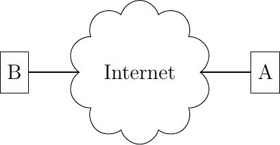
Throughout this part, we will consider the Internet as a black box as shown in Fig. 6. We will focus on hos hosts interact and will reveal how the network really operates in the second part of the book.

Fig. 6 Internet hosts can exchange packets

Thanks to these architectural principles, any Internet host can send an IP packet at any time to any other Internet host. A host could send a packet to a server in America and shortly after another packet to a server in Australia or Africa. For a host, sending a packet is a cheap operation. It creates a sequence of bytes containing the header and the payload and then passes it to the network interface card. The other elements of the network will handle the packet and deliver it to its final destination.

A primer on IP version 4

Two different versions of the Internet protocol are used on today’s Internet. The first one, named IP version 4 uses 32-bit long addresses. IPv4 addresses are often represented in dotted-decimal format as a sequence of four integers separated by a dot. The first integer is the decimal representation of the most significant byte of the 32-bit IPv4 address, … For example,

• 1.2.3.4 corresponds to 00000001 00000010 00000011 00000100

• 127.0.0.1 corresponds to 01111111 00000000 00000000 00000001

• 255.255.255.255 corresponds to 1111111 1111111 11111111 1111111111

This version was designed when the Internet was a research network that connected computers in universities and research labs. At that time, having a maximum of \(2^{32}\) IPv4 addresses was not considered to be a severe limitation. Today, almost all the available IPv4 addresses have been assigned to various organizations ranging from enterprises or universities to Internet Service Providers.

An IPv4 address is composed of two parts : a subnetwork identifier and a host identifier. The subnetwork identifier is composed of the high-order bits of the address, and the host identifier is encoded in the low-order bits of the address. This is illustrated in figure Fig. 7 with a 22-bit subnetwork identifier shown in blue and a 12-bit host identifier in red.

Fig. 7 The subnetwork (blue) and host identifiers (red) inside an IPv4 address

Flexibility in the IPv4 addressing architecture was added with the introduction of variable-length subnets in RFC 1519. IPv4 supports variable-length subnets where the subnet identifier can be any size, from 1 to 31 bits. Variable-length subnets allow the network operators to use a subnet that better matches the number of hosts that are placed inside the subnet. A subnet identifier or IPv4 prefix is usually represented as A.B.C.D/p where A.B.C.D is the network address obtained by concatenating the subnet identifier with a host identifier containing only 0 and p is the length of the subnet identifier in bits. The table below provides examples of IP subnets.

Subnet	Number of addresses	Smallest address	Highest address
10.0.0.0/8	16,777,216	10.0.0.0	10.255.255.255
192.168.0.0/16	65,536	192.168.0.0	192.168.255.255
198.18.0.0/15	131,072	198.18.0.0	198.19.255.255
192.0.2.0/24	256	192.0.2.0	192.0.2.255
10.0.0.0/30	4	10.0.0.0	10.0.0.3
10.0.0.0/31	2	10.0.0.0	10.0.0.1

Note

Special IPv4 addresses

Most unicast IPv4 addresses can appear as source and destination addresses in packets on the global Internet. However, it is worth noting that some blocks of IPv4 addresses have a special usage, as described in RFC :5735. These include :

• 0.0.0.0/8, which is reserved for self-identification. A common address in this block is 0.0.0.0, which is sometimes used when a host boots and does not yet know its IPv4 address.

• 127.0.0.0/8, which is reserved for loopback addresses. Each host implementing IPv4 must have a loopback interface (that is not attached to a datalink layer). By convention, IPv4 address 127.0.0.1 is assigned to this interface. This allows processes running on a host to use TCP/IP to contact other processes running on the same host. This can be very useful for testing purposes.

• 10.0.0.0/8, 172.16.0.0/12, and 192.168.0.0/16 are reserved for private networks that are not directly attached to the Internet. These addresses are often called private addresses or RFC 1918 addresses.

• 169.254.0.0/16 is used for link-local addresses RFC 3927. Some hosts use an address in this block when they are connected to a network that does not allocate addresses as expected.

• 192.0.2.0/24, 198.51.100.0/24, and 203.0.113.0/24 are reserved for use in documentation. These addresses cannot be used on the public Internet and should not be accepted by hosts. This book should ideally use these addresses when providing examples.

The unit of information for IPv4 is the packet. An IPv4 packet has a 20-byte header which contains the source and destination addresses of the packet and some control information. One of the control fields of the IPv4 header is a 16-bit field that contains the total length of the packet (header included). An IPv4 packet cannot be longer than 65535 bytes, header included. In practice, hosts rarely send really long packets and most IPv4 packets are shorter than about 1500 bytes. The IPv4 packet header is shown in Fig. 8.

Fig. 8 The IP version 4 header

A primer on IP version 6

The second deployed version of IP is IP version 6. This version of IP introduces several changes compared to IP version 4 that will be discussed later. The most important one is the length of the IPv6 addresses. An IPv6 address is 128 bits long. This implies that in theory, there are \(2^128=340,282,366,920,938,463,463,374,607,431,768,211,456\) unique IPv6 addresses. The number of IPv6 addresses is much larger than the number of IPv4 addresses, and we do not expect the IPv6 addressing space to become exhausted one day.

Note

Textual representation of IPv6 addresses

It is sometimes necessary to write IPv6 addresses in text format, e.g. when manually configuring addresses or for documentation purposes. The preferred format for writing IPv6 addresses is x:x:x:x:x:x:x:x, where the x ‘s are hexadecimal digits representing the eight 16-bit parts of the address. Here are a few examples of IPv6 addresses :

• abcd:ef01:2345:6789:abcd:ef01:2345:6789

• 2001:db8:0:0:8:800:200c:417a

• fe80:0:0:0:219:e3ff:fed7:1204

IPv6 addresses often contain a long sequence of bits set to 0. In this case, a compact notation has been defined. With this notation, :: is used to indicate one or more groups of 16-bit blocks containing only bits set to 0. For example,

• 2001:db8:0:0:8:800:200c:417a is represented as 2001:db8::8:800:200c:417a

• ff01:0:0:0:0:0:0:101 is represented as ff01::101

• 0:0:0:0:0:0:0:1 is represented as ::1

• 0:0:0:0:0:0:0:0 is represented as ::

An IPv6 prefix can be represented as address/length, where length is the length of the prefix in bits. For example, the three notations below correspond to the same IPv6 prefix :

• 2001:0db8:0000:cd30:0000:0000:0000:0000 / 60

• 2001:0db8::cd30:0:0:0:0 / 60

• 2001:0db8:0:cd30:: / 60

An IPv6 packet starts with a header of at least 40 bytes. It contains the source and destination IPv6 addresses as well as a 16-bit-long length field. This implies that IPv6 packets cannot be longer than 65535 bytes. As for IPv4, most observed IPv6 packets are shorter than about 1500 bytes.

The standard IPv6 header defined in RFC 2460 occupies 40 bytes and contains 8 different fields, as shown in Fig. 9. The structure of this packet will be explained in more detail in the second part of this book.

Fig. 9 The IP version 6 header

The transport layer

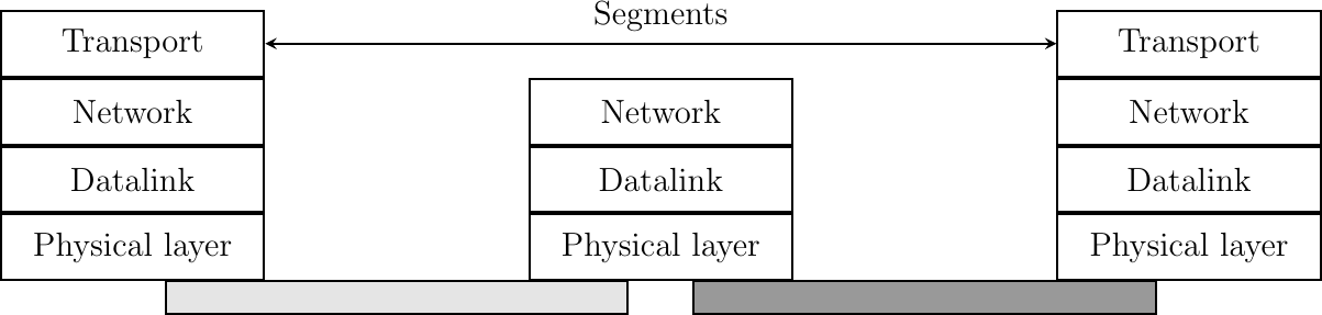
The network layer enables hosts to reach each others through intermediate routers. However, different communication flows can take place between the same hosts. These communication flows might have different needs (some require reliable delivery, other not) and need to be distinguished. Ensuring an identification of a communication flow between two given hosts is the task of the transport layer. Transport layer entities exchange segments. A segment is a finite sequence of bytes that are transported inside one or more packets. A transport layer entity issues segments (or sometimes part of segments) as Data.request to the underlying network layer entity. This is illustrated in Fig. 10.

There are different types of transport layers. The most widely used transport layers on the Internet are TCP, that provides a reliable connection-oriented bytestream transport service, and UDP, that provides an unreliable connection-less transport service.

Fig. 10 The transport layer

A network is always designed and built to enable applications running on hosts to exchange information. In a previous chapter, we have explained the principles of the network layer that enables hosts connected to different types of datalink layers to exchange information through routers. These routers act as relays in the network layer and ensure the delivery of packets between any pair of hosts attached to the network.

The network layer ensures the delivery of packets on a hop-by-hop basis through intermediate nodes. As such, it provides a service to the upper layer. In practice, this layer is usually the transport layer that improves the service provided by the network layer to make it usable by applications. This is illustrated in Fig. 11.

Fig. 11 The transport layer

Most networks use a datagram organization and provide a simple service which is called the connectionless service.

As the transport layer is built on top of the network layer, it is important to know the key features of the network layer service. In this book, we only consider the connectionless network layer service which is the most widespread. Its main characteristics are :

• the connectionless network layer service can only transfer SDUs of limited size

• the connectionless network layer service may discard SDUs

• the connectionless network layer service may corrupt SDUs

• the connectionless network layer service may delay, reorder or even duplicate SDUs

These imperfections of the connectionless network layer service are caused by the operations of the network layer. This layer is able to deliver packets to their intended destination, but it cannot guarantee their delivery. The main cause of packet losses and errors are the buffers used on the network nodes. If the buffers of one of these nodes becomes full, all arriving packets must be discarded. This situation frequently happens in practice. Transmission errors can also affect packet transmissions on links where reliable transmission techniques are not enabled or because of errors in the buffers of the network nodes.

There are three main types of transport services :

• the connectionless service

• the connection-oriented (byte-stream or message-mode) service

• the request-response service

The connectionless transport service

The connectionless service allows applications to easily exchange messages or Service Data Units. On the Internet, this service is provided by the UDP protocol that will be explained in the next chapter. The connectionless transport service on the Internet is unreliable, but is able to detect transmission errors. This implies that an application will not receive data that has been corrupted due to transmission errors.

The figure below provides a representation of the connectionless service as a time-sequence diagram. The user on the left, having address S, issues a Data.request primitive containing Service Data Unit (SDU) M that must be delivered by the service provider to destination D. The dashed line between the two primitives indicates that the Data.indication primitive that is delivered to the user on the right corresponds to the Data.request primitive sent by the user on the left.

There are several possible implementations of the connectionless service. Before studying these realizations, it is useful to discuss the possible characteristics of the connectionless service. A reliable connectionless service is a service where the service provider guarantees that all SDUs submitted in Data.requests by a user will eventually be delivered to their destination. Such a service would be very useful for users, but guaranteeing perfect delivery is difficult in practice. For this reason, network layers usually support an unreliable connectionless service.

An unreliable connectionless service may suffer from various types of problems compared to a reliable connectionless service. First of all, an unreliable connectionless service does not guarantee the delivery of all SDUs. This can be expressed graphically by using the time-sequence diagram below.

In practice, an unreliable connectionless service will usually deliver a large fraction of the SDUs. However, since the delivery of SDUs is not guaranteed, the user must be able to recover from the loss of any SDU.

A second imperfection that may affect an unreliable connectionless service is that it may duplicate SDUs. Some packets may be duplicated in a network and be delivered twice to their destination. This is illustrated by the time-sequence diagram below.

Finally, some unreliable connectionless service providers may deliver to a destination a different SDU than the one that was supplied in the Data.request. This is illustrated in the figure below.

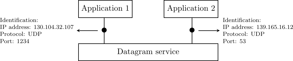
The connectionless transport service allows networked application to exchange messages. Several networked applications may be running at the same time on a single host. Each of these applications must be able to exchange SDUs with remote applications. To enable these exchanges of SDUs, each networked application running on a host is identified by the following information :

• the host on which the application is running

• the port number on which the application listens for data

On the Internet, the port number is an integer and the host is identified by its IPv4 or IPv6 address. A host that only has an IPv4 address cannot communicate with a host having only an IPv6 address. Fig. 12 illustrates two applications that are using the datagram service provided by UDP on hosts that are using IPv4 addresses.

Fig. 12 The connectionless or datagram service

The connection-oriented transport service

An invocation of the connection-oriented service is divided into three phases. The first phase is the establishment of a connection. A connection is a temporary association between two users through a service provider. Several connections may exist at the same time between any pair of users. Once established, the connection is used to transfer SDUs. Connections usually provide one bidirectional stream supporting the exchange of SDUs between the two users that are associated through the connection. This stream is used to transfer data during the second phase of the connection called the data transfer phase. The third phase is the termination of the connection. Once the users have finished exchanging SDUs, they request the service provider to terminate the connection. As we will see later, there are also some cases where the service provider may need to terminate a connection itself.

The establishment of a connection can be modeled by using four primitives : Connect.request, Connect.indication, Connect.response and Connect.confirm. The Connect.request primitive is used to request the establishment of a connection. The main parameter of this primitive is the address of the destination user. The service provider delivers a Connect.indication primitive to inform the destination user of the connection attempt. If it accepts to establish a connection, it responds with a Connect.response primitive. At this point, the connection is considered to be established and the destination user can start sending SDUs over the connection. The service provider processes the Connect.response and will deliver a Connect.confirm to the user who initiated the connection. The delivery of this primitive terminates the connection establishment phase. At this point, the connection is considered to be open and both users can send SDUs. A successful connection establishment is illustrated below.

The example above shows a successful connection establishment. However, in practice not all connections are successfully established. One reason is that the destination user may not agree, for policy or performance reasons, to establish a connection with the initiating user at this time. In this case, the destination user responds to the Connect.indication primitive by a Disconnect.request primitive that contains a parameter to indicate why the connection has been refused. The service provider will then deliver a Disconnect.indication primitive to inform the initiating user.

A second reason is when the service provider is unable to reach the destination user. This might happen because the destination user is not currently attached to the network or due to congestion. In these cases, the service provider responds to the Connect.request with a Disconnect.indication primitive whose reason parameter contains additional information about the failure of the connection.

Once the connection has been established, the service provider supplies two data streams to the communicating users. The first data stream can be used by the initiating user to send SDUs. The second data stream allows the responding user to send SDUs to the initiating user. The data streams can be organized in different ways. A first organization is the message-mode transfer. With the message-mode transfer, the service provider guarantees that one and only one Data.indication will be delivered to the endpoint of the data stream for each Data.request primitive issued by the other endpoint. The message-mode transfer is illustrated in the figure below. The main advantage of the message-transfer mode is that the recipient receives exactly the SDUs that were sent by the other user. If each SDU contains a command, the receiving user can process each command as soon as it receives a SDU.

Unfortunately, the message-mode transfer is not widely used on the Internet. On the Internet, the most popular connection-oriented service transfers SDUs in stream-mode. With the stream-mode, the service provider supplies a byte stream that links the two communicating users. The sending user sends bytes by using Data.request primitives that contain sequences of bytes as SDUs. The service provider delivers SDUs containing consecutive bytes to the receiving user by using Data.indication primitives. The service provider ensures that all the bytes sent at one end of the stream are delivered correctly in the same order at the other endpoint. However, the service provider does not attempt to preserve the boundaries of the SDUs. There is no relation enforced by the service provider between the number of Data.request and the number of Data.indication primitives. The stream-mode is illustrated in the figure below. In practice, a consequence of the utilization of the stream-mode is that if the users want to exchange structured SDUs, they will need to provide the mechanisms that allow the receiving user to separate successive SDUs in the byte stream that it receives. Application layer protocols often use specific delimiters such as the end of line character to delineate SDUs in a bytestream.

The third phase of a connection is its release. As a connection involves three parties (two users and one service provider), any of them can request the termination of the connection. Usually, connections are terminated upon request of one user once the data transfer is finished. However, sometimes the service provider may be forced to terminate a connection. This can be due to lack of resources inside the service provider or because one of the users is not reachable anymore through the network. In this case, the service provider will issue Disconnect.indication primitives to both users. These primitives will contain, as parameter, some information about the reason for the termination of the connection. Unfortunately, as illustrated in the figure below, when a service provider is forced to terminate a connection it cannot guarantee that all SDUs sent by each user have been delivered to the other user. This connection release is said to be abrupt as it can cause losses of data.

An abrupt connection release can also be triggered by one of the users. If a user needs, for any reason, to terminate a connection quickly, it can issue a Disconnect.request primitive and to request an abrupt release. The service provider will process the request, stop the two data streams and deliver the Disconnect.indication primitive to the remote user as soon as possible. As illustrated in the figure below, this abrupt connection release may cause losses of SDUs.

To ensure a reliable delivery of the SDUs sent by each user over a connection, we need to consider the two streams that compose a connection as independent. A user should be able to release the stream that it uses to send SDUs once it has sent all the SDUs that it planned to send over this connection, but still continue to receive SDUs over the opposite stream. This graceful connection release is usually performed as shown in the figure below. One user issues a Disconnect.request primitive to its provider once it has issued all its Data.request primitives. The service provider will wait until all Data.indication primitives have been delivered to the receiving user before issuing the Disconnnect.indication primitive. This primitive informs the receiving user that it will no longer receive SDUs over this connection, but it is still able to issue Data.request primitives on the stream in the opposite direction. Once the user has issued all of its Data.request primitives, it issues a Disconnnect.request primitive to request the termination of the remaining stream. The service provider will process the request and deliver the corresponding Disconnect.indication to the other user once it has delivered all the pending Data.indication primitives. At this point, all data has been delivered, the two streams have been released successfully and the connection is completely closed.

Note

Reliability of the connection-oriented service

An important point to note about the connection-oriented service is its reliability. A connection-oriented service can only guarantee the correct delivery of all SDUs provided that the connection has been released gracefully. This implies that while the connection is active, there is no guarantee for the actual delivery of the SDUs exchanged as the connection may need to be abruptly released at any time.

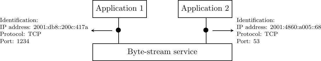
The second transport service is the connection-oriented service. On the Internet, this service is often called the byte-stream service as it creates a reliable byte stream between the two applications that are linked by a transport connection. Like the datagram service, the networked applications that use the byte-stream service are identified by the host on which they run and a port number. These hosts can be identified by an address or a name. Fig. 13 illustrates two applications that are using the byte-stream service provided by the TCP protocol on IPv6 hosts. The byte-stream service provided by TCP is reliable and bidirectional.

Fig. 13 The connection-oriented or byte-stream service

The request-response service

The request-response service is a compromise between the connectionless service and the connection-oriented service. Many applications need to send a small amount of data and receive a small amount of information back. This is similar to procedure calls in programming languages. A call to a procedure takes a few arguments and returns a simple answer. In a network, it is sometimes useful to execute a procedure on a different host and receive the result of the computation. Executing a procedure on another host is often called Remote Procedure Call. It is possible to use the connectionless service for this application. However, since this service is usually unreliable, this would force the application to deal with any type of error that could occur. Using the connection oriented service is another alternative. This service ensures the reliable delivery of the data, but a connection must be created before the beginning of the data transfer. This overhead can be important for applications that only exchange a small amount of data.

The request-response service allows to efficiently exchange small amounts of information in a request and associate it with the corresponding response. This service can be depicted by using the time-sequence diagram below.

Note

Services and layers

In the previous sections, we have described services that are provided by the transport layer. However, it is important to note that the notion of service is more general than in the transport layer. As explained earlier, the network layer also provides a service, which in most networks is an unreliable connectionless service. There are network layers that provide a connection-oriented service. Similarly, the datalink layer also provides services. Some datalink layers will provide a connectionless service. This will be the case in Local Area Networks for examples. Other datalink layers, e.g. in public networks, provide a connection oriented service.

The transport layer

The transport layer entity interacts with both a user in the application layer and the network layer. It improves the network layer service to make it usable by applications. From the application’s viewpoint, the main limitations of the network layer service come from its unreliable service:

• the network layer may corrupt data;

• the network layer may loose data;

• the network layer may not deliver data in-order;

• the network layer has an upper bound on maximum length of the data;

• the network layer may duplicate data.

To deal with these issues, the transport layer includes several mechanisms that depend on the service that it provides. It interacts with both the applications and the underlying network layer.

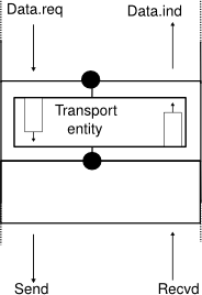
Fig. 14 Interactions between the transport layer, its user, and its network layer provider

We have already described in the datalink layers mechanisms to deal with data losses and transmission errors. These techniques are also used in the transport layer.

Connectionless transport

The simplest service that can be provided in the transport layer is the connectionless transport service. Compared to the connectionless network layer service, this transport service includes two additional features :

• an error detection mechanism that allows detecting corrupted data

• a multiplexing technique that enables several applications running on one host to exchange information with another host

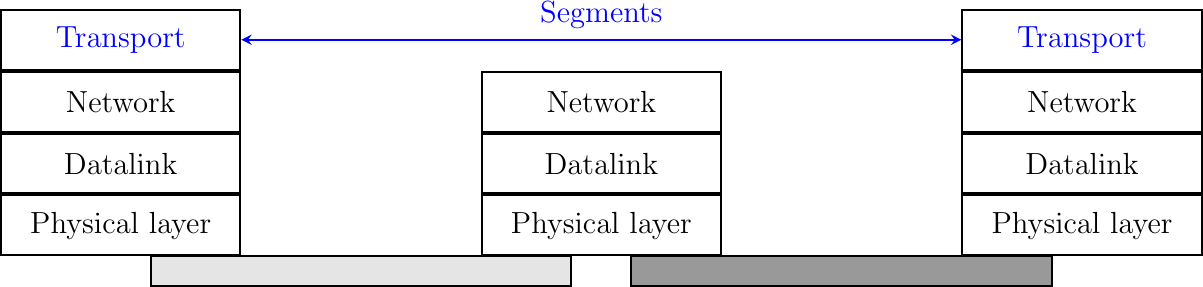
To exchange data, the transport protocol encapsulates the SDU produced by its user inside a segment. The segment is the unit of transfer of information in the transport layer. Transport layer entities always exchange segments. When a transport layer entity creates a segment, this segment is encapsulated by the network layer into a packet which contains the segment as its payload and a network header. The packet is then encapsulated in a frame to be transmitted in the datalink layer.

Fig. 15 Segments are the unit of transfer at transport layer

A segment also contains control information, usually stored inside a header and the payload that comes from the application. To detect transmission errors, transport protocols rely on checksums or CRCs like the datalink layer protocols.

Compared to the connectionless network layer service, the transport layer service allows several applications running on a host to exchange SDUs with several other applications running on remote hosts. Let us consider two hosts, e.g. a client and a server. The network layer service allows the client to send information to the server, but if an application running on the client wants to contact a particular application running on the server, then an additional addressing mechanism is required. The network layer address identifies a host, but it is not sufficient to differentiate the applications running on a host. Port numbers provides this additional addressing. When a server application is launched on a host, it registers a port number. This port number will be used by the clients to contact the server process.

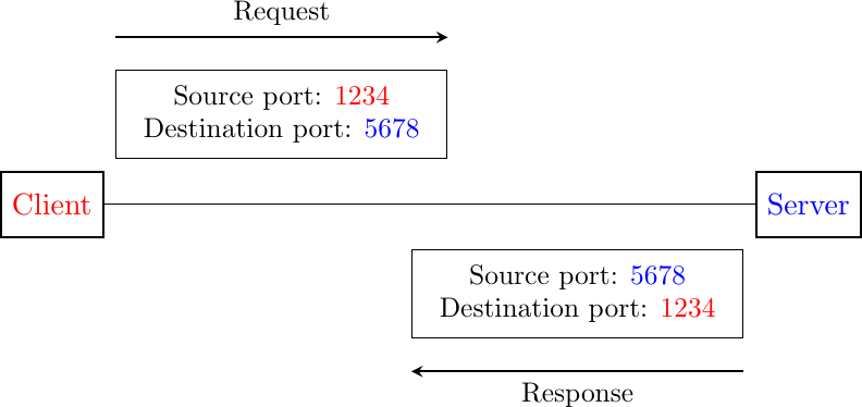
The figure below shows a typical usage of port numbers. The client process uses port number 1234 while the server process uses port number 5678. When the client sends a request, it is identified as originating from port number 1234 on the client host and destined to port number 5678 on the server host. When the server process replies to this request, the server’s transport layer returns the reply as originating from port 5678 on the server host and destined to port 1234 on the client host.

Fig. 16 Utilization of port numbers

The User Datagram Protocol

The User Datagram Protocol (UDP) is defined in RFC 768. It provides an unreliable connectionless transport service on top of the unreliable network layer connectionless service. The main characteristics of the UDP service are :

• the UDP service cannot deliver SDUs that are larger than 65467 bytes [1]

• the UDP service does not guarantee the delivery of SDUs (losses can occur and SDUs can arrive out-of-sequence)

• the UDP service will not deliver a corrupted SDU to the destination

Compared to the connectionless network layer service, the main advantage of the UDP service is that it allows several applications running on a host to exchange SDUs with several other applications running on remote hosts. Let us consider two hosts, e.g. a client and a server. The network layer service allows the client to send information to the server, but if an application running on the client wants to contact a particular application running on the server, then an additional addressing mechanism is required other than the IP address that identifies a host, in order to differentiate the application running on a host. This additional addressing is provided by port numbers. When a server using UDP is enabled on a host, this server registers a port number. This port number will be used by the clients to contact the server process via UDP.

Figure Fig. 17 shows a typical usage of the UDP port numbers. The client process uses port number 1234, while the server process uses port number 5678. When the client sends a request, it is identified as originating from port number 1234 on the client host and destined to port number 5678 on the server host. When the server process replies to this request, the server’s UDP implementation will send the reply as originating from port 5678 on the server host and destined to port 1234 on the client host.

Fig. 17 Usage of the UDP port numbers

UDP uses a single segment format shown in figure Fig. 18.

Fig. 18 UDP Header Format

The UDP header contains four fields :

• a 16-bit source port

• a 16-bit destination port

• a 16-bit length field

• a 16-bit checksum

As the port numbers are encoded as a 16-bit field, there can be up to only 65535 different server processes that are bound to a different UDP port at the same time on a given server. In practice, this limit is never reached. However, it is worth noticing that most implementations divide the range of allowed UDP port numbers into three different ranges :

• the privileged port numbers (1 < port < 1024 )

• the ephemeral port numbers ( officially [2] 49152 <= port <= 65535 )

• the registered port numbers (officially 1024 <= port < 49152)

In most Unix variants, only processes having system administrator privileges can be bound to port numbers smaller than 1024. Well-known servers such as DNS, NNTP,or RPC use privileged port numbers. When a client needs to use UDP, it usually does not require a specific port number. In this case, the UDP implementation will allocate the first available port number in the ephemeral range. The range of registered port numbers should be used by servers. In theory, developers of network servers should register their port number officially through IANA [3], but few developers do this.

UDP can be used over IPv4 or IPv6. When a host receives an IP packet, it needs to determine whether this packet should be processed by UDP or another transport protocol. This is done by using the Protocol field in the IP version 4 header. The Internet Assigned Numbers Authority (IANA) maintains a registry of the assigned Internet Protocol numbers that assigns one integer to each protocol which can be carried inside an IP packet. This registry specifies that 17 is reserved to indicate a UDP segment. Figure Fig. 19 shows a UDP segment inside an IPv4 packet.

Fig. 19 An IPv4 packet containing an empty UDP segment

Note

Computation of the UDP checksum

Many Internet protocols use the Internet checksum defined in RFC 1071 to detect transmission errors. This checksum is computed by the sender and verified by the received. The algorithm defined in RFC 1071 uses modular arithmetic. It is computed over a sequence of bytes which is padded if it contains an odd number of bytes. The checksum is the one’s complement of the sum of the 16 bits words modulo \(2^16\). The python code below computes the Internet checksum.

def internet_checksum(data: bytes) -> int:
    """
    Compute the Internet Checksum of the supplied data.
    :param data: The input data as bytes
    :return: The checksum as an integer (16-bit)
    """
    if len(data) % 2:
      data += b'\x00'  # pad to even length

    checksum = 0
    for i in range(0, len(data), 2):
        word = (data[i] << 8) + data[i+1]
        checksum += word
        # carry around
        checksum = (checksum & 0xFFFF) + (checksum >> 16)

    return ~checksum & 0xFFFF  # one's complement


# Example usage
if __name__ == "__main__":
    test_data = b"a sequence of bytes"
    chk = internet_checksum(test_data)
    print(f"Checksum: 0x{chk:04X}")

The byte array used to compute the checksum of an UDP segment contains :

• a pseudo header RFC 2460 containing the source address, the destination address, the packet length encoded as a 32-bit number and a 32-bit bit field containing the three most significant bytes set to 0 and the low-order byte set to 17

• the entire UDP segment, including its header

Several types of applications rely on UDP. As a rule of thumb, UDP is used for applications where delay must be minimized or losses can be recovered by the application itself. A first-class of UDP-based applications are applications where the client sends a short request and expects a quick and short answer. The DNS is an example of a UDP application that is often used in the wide area. However, in local area networks, many distributed systems rely on Remote Procedure Call (RPC) that is often used on top of UDP. In Unix environments, the Network File System (NFS) is built on top of RPC and runs frequently on top of UDP. A second class of UDP-based applications are the interactive computer games that need to frequently exchange small messages, such as the player’s location or their recent actions. Many of these games use UDP to minimize the delay and can recover from losses. A third class of applications are multimedia applications such as interactive Voice over IP or interactive Video over IP. These interactive applications expect a delay shorter than about 200 milliseconds between the sender and the receiver and can recover from losses directly inside the application.

Footnotes

[1]

This limitation is due to the fact that the network layer cannot transport packets that are larger than 64 KBytes. As UDP does not include any segmentation/reassembly mechanism, it cannot split a SDU before sending it. The UDP header consumes 8 bytes and the IPv6 header 60. With IPv4, the IPv4 header only consumes 20 bytes and thus the maximum UDP payload size is 65507 bytes.

[2]

A discussion of the ephemeral port ranges used by different TCP/UDP implementations may be found in http://www.ncftp.com/ncftpd/doc/misc/ephemeral_ports.html

[3]

The complete list of allocated port numbers is maintained by IANA . It may be downloaded from http://www.iana.org/assignments/port-numbers